Hey there 👋
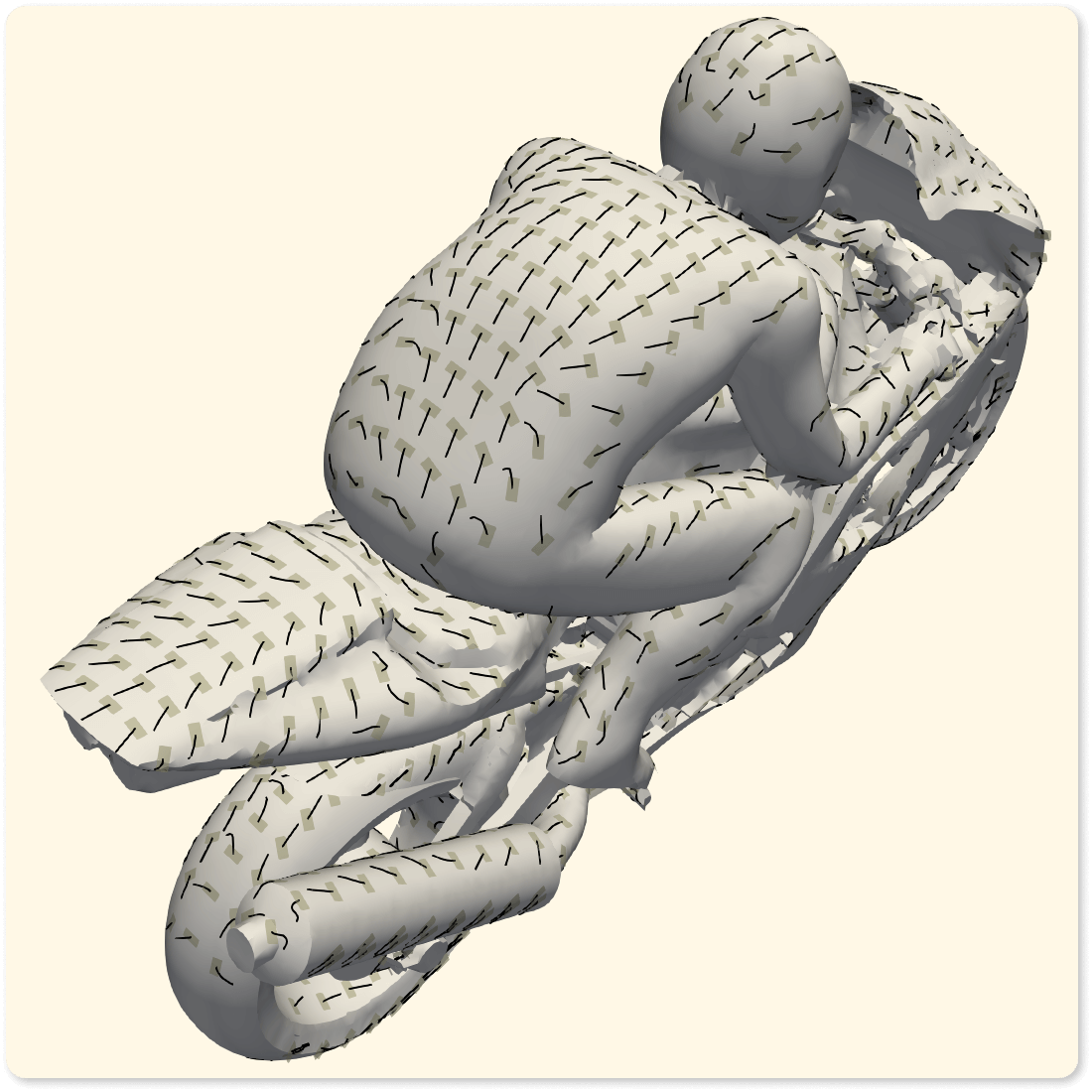
It’s Robin from CFD Engine and we’re making plots like this today 👇

Customisable virtual wool tufts, all done in ParaView (including the sticky tape).
They’re a simple, intuitive (& surprisingly informative) way to show local flow alignment.
They get even better if you have transient data. Set them up, animate through your timesteps & watch them wobble around in regions of separated/unsteady flow.
They’ve been a staple of experimental testing for ever & now you can add them to your CFD toolkit.
Let’s go…
The basics
The wool tufts are forward-traced streamlines, restricted to the model surface & capped to stay short.
The sticky-tape strips are 2D square glyphs, scaled a little wider & rotated to lay on the surface.
They’re both placed on a regular(ish) grid made by chopping the model surfaces with a bunch of 2D slices.
So, other than ParaView, all you’ll need is a CFD result with some near-wall velocity (or wall shear stress) data.
I usually export near-wall velocity using the nearWallFields function object (there are examples in the cavity & motorBike tutorials, should you need them).
The specifics
Prep
With your simulation data loaded & your surfaces at the ready, start by applying a Generate Surface Normals filter (the normals will make your surfaces look smoother & we’ll need them later for the sticky tape).
Spaced out
Next up, apply the slice filter to the Generate Surface Normals result. In my case, I used a plane slice, set the origin to zero, set the normal to X & added 50+ locations using the value range option. You’ll end up with a series of outlines in a single result.
Next up, slice your slices. Take the output from the previous step & repeat your slicing in a different direction. I used a Y-normal slice, but a Z-normal would’ve worked just as well.
We’re slicing lines this time (as opposed to surfaces) & so we’ll end up with a bunch of nicely-spaced points.
We’ll use these points as the origin for our tufts & to place our tape.
Tufts
On to the tufts. Add a Stream Tracer with Custom Source using the result of Generate Surface Normals as its input & the second slice filter as its seed.
Trace forward-streamlines using your near-wall velocity field (or wall shear field) making sure you click the box to request surface streamlines. Tweak the maximum streamline length to make them nice & short.
Tape
The tape is more than just a fun addition. We need something to indicate the origin of our tufts & therefore indicate the direction of the flow. We might as well make them look like sticky tape while we’re at it.
Select the second slice filter (the one with the points) & apply a Glyph filter. Set it to a 2D square glyph & set the orientation to Normals. Turn off the scale array & set a scale factor that looks good.
The tape is probably normal to the surface at this point. Rotate it using the transform built into the glyph filter. I rotated my glyphs 90º about the Y-axis (to lay them on the surface) & scaled them in the X & Y directions to make them less square.
That’s it
Show your Generate Surface Normals result as a surface. The streamlines are your tufts & the glyphs are your tape. Colour them appropriately & save a state file (so you don’t have to do it all again).
If your original dataset has several timesteps, press play & watch your tufts wobble around in the breeze.
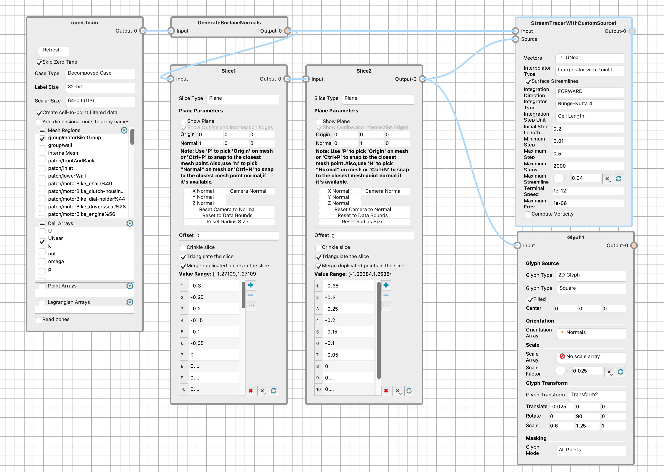
Here’s a node diagram that shows all the details of the pipeline (click for a readable version).

You don’t need to build anything using the node editor, it’s just a neat way of showing the filters, their settings & how they’re linked – all in a single image.
Go for it
You probably won’t need wool tufts everyday, but they have their place.
Would I use them to make development decisions? No.
Would I show them to non-technical stakeholders to explain why their new product is better? Yes.
They’re a bit of fun too, which is a bonus 🙌
Let me know what you reckon, especially if you give them a go. I’m keen to see how they turn out on your models 🤞
Until next time, stay safe,
