Hey there,
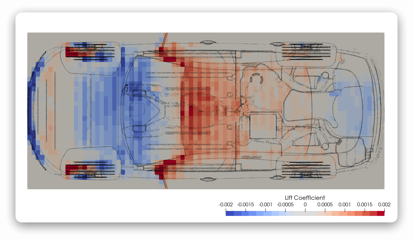
It’s Robin from CFD Engine & I’m back with some tricks to get last week’s force bins into ParaView so that you can plot an 8-bit masterpiece like this one 👇

In case you’re wondering, it’s a lift-force X-ray of the drivAer model, where the lifting bits are red & the downforcing bits are blue (it’s the same plot as last time – I’m lazy).
I gave you the back story in last week’s email & shared an example dictionary, so that you could export force “bins” from the motorBike tutorial. This week we’re wrangling that data into ParaView 🤞
But, in case you missed it, here’s a recap…
Catch Up
This technique takes advantage of a new function object in OpenFOAM v2206 – binField – which lets us chop our model into segments & report the forces acting on those segments. By presenting this data as a planar heatmap, we can reveal our model’s force distribution in a single view, with nothing obscured (a bit like an X-ray).
Creating the data is pretty straight-forward, using it is more of a challenge. The raw binField data won’t go straight into ParaView (wrong format), nor will it import into Excel (too many columns) – we need a workaround 🤔
How do we go from raw binField data, to a plot in ParaView?
Overview
We’re going to get ParaView do the hard work for us by making a planar grid, complete with connectivity & cell data, which we’ll later swap out for our own.
Before we get started, read your binField .dat file (found under the postProcessing/binField directory) into a text editor for reference.
Step 01: Create a Plane in ParaView
In an empty ParaView session, use the Plane source filter to create a new object (Sources > Geometric Shapes > Plane).
If you’ve not used this filter before:
Originis typically (Xmin,Ymin,Zmin)Point1is the other end of the x-axis (Xmax,Ymin,Zmin)Point2is the other end of the y-axis (Xmin,Ymax,Zmin)X & Y resolutionare the number of cells in each direction
We can get all of these values from the first few lines of our binField output file. e0 bins is our X-resolution, e0 bins start is our Xmin value & e0 bins end is our Xmax value.
Similarly, e1 has the Y axis data, whilst e2 has the Z data (should we need it).
Step 02: Add some dummy data
Select the Plane you just created & apply the Append Location Attributes filter.
This will add a few new fields, one of which is CellCenters, a single value for each cell which we’ll use as a placeholder for our own data.
Step 03: Write it out
Select the AppendLocationAttributes object in the pipeline.
Click File > Save Data, give it a name, set the file type to Legacy VTK files (*.vtk)* & click OK to bring up the next dialog.
We only want the CellCenters field so click the Choose Arrays to Write checkbox & deselect the other fields.
Change the format to Ascii (so that we can edit it in a text editor later) & click OK to save.
We now have an editable data file, with a planar grid that corresponds to our binField settings, plus a dummy cell-based dataset ready to be swapped out.
Step 04: Juggle the binField data
Back to the binField data in our text editor.
The file format isn’t super-friendly, we’ve got 21 header lines detailing the bin settings, followed by a line of column names & a line of data. We need to:
- Strip the header info (delete top 21 lines);
- Delete the
#symbol & space from in front of “Time”; - Copy & Paste the remaining data into the text box at the top of this awesome online converter – which will (🤞)
- reformat the data into a proper CSV format;
- convert it from columns to rows;
- filter the rows (in 2 steps) leaving just the
total _Zrows; - extract the force data column, ready to be copied to clipboard (see the last blue box on the page).
You could do all of the above with Unix tools, or Perl, or Python, but that website is super-handy 👍👍
Step 05: Replace the dummy data
Read the VTK datafile from Step 03 into a text editor and search for CellCenters
Replace the block of data below it (including the Metadata section) with the output from Step 04.
You can change the field’s name from CellCenters to something more descriptive (Force Coeff Z) if you like.
Save it as a new VTK file.
Step 06: Read into ParaView
Read that new VTK file into ParaView & make your plot.
Here are a couple of tips:
- use a 2D view to avoid perspective issues.
- overlay the model geometry (displayed semi-transparent or as feature edges) to help with locating areas of interest.
- use a diverging colourmap (like the default cool-to-warm map) & centre the range on zero so that segments with negligible force are de-emphasised.
If you’re doing several force x-rays that all use the same bin configuration, then you’ll probably only need to repeat Steps 04–06, swapping in your new force data each time.
In the bin?
In case you hadn’t noticed, this isn’t slick or polished & it’s not “production ready” 🙈 It’s a first-draft recipe for handcrafting a few force X-ray plots to see if they’re as useful as I suggested.
Will you try it? Probably not, but there are a few handy hints in these emails and, if nothing else, the conversion website is well worth exploring.
Drop me a screenshot if you make it work (or if you find a better workflow) I’d be keen to see your results.
Until next week, stay safe,
